This is part of series of posts about associative grouping:
- Part 1 - Associative Grouping using tSQL Recursive CTE’s
- Part 2 - Associative Grouping using tSQL Graph
In the first two parts of this series we looked at how we could use recursive CTE’s and SQL Server’s graph functionality to find overlapping groups in two columns in a table, in order to put them into a new super group of associated groups.
Since then I’ve been doing most of my work in Azure, and doing quite a lot with Databricks/Spark. I recently responded to a tweet about trying to do what we had done in the first tow posts. It transpired that they were using Synapse SQL pools, so neither of the previous methods were supported.
I've records with an 'Id' and a 'Best Match Id' and I want to create 1 logical cluster for easier filter on the data set
— Johannes Vink (@JohannesVink) September 27, 2021
This is a clean data set, but an 'Id' can refer to a different cluster
I need hints on how to solve this. Google returns MERGE/clustered indexes... #sqlhelp pic.twitter.com/EVv35dF48p
This got me thinking, if you’re working with data lakes and/or Azure Synapse SQL Pools, how would you go about doing this? We can use the GraphFrames library in Databricks to process the data and find the groups for us.
Installing the Library
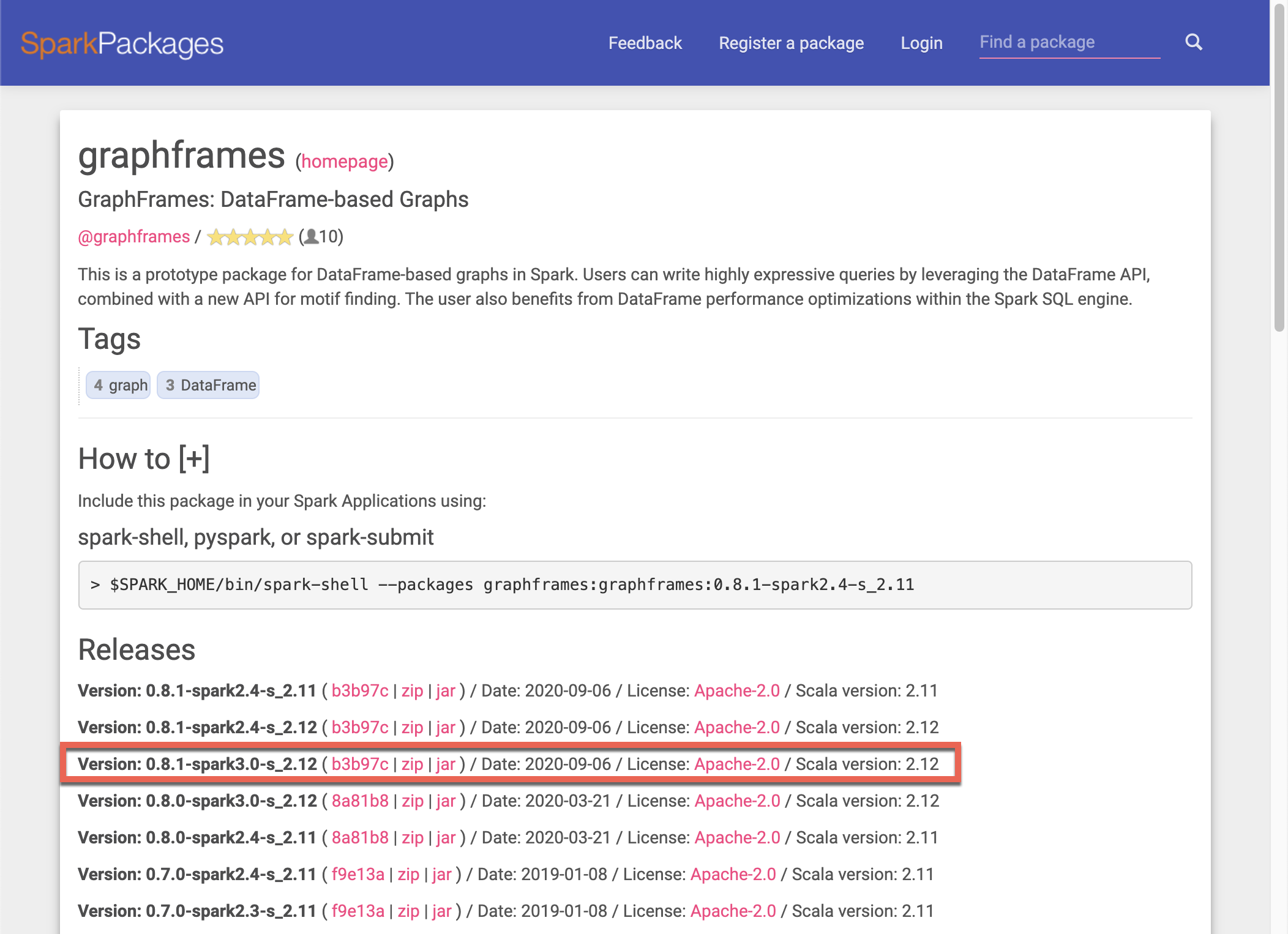
First we need to download the GraphFrames library. I’m using a Databricks cluster with spark 3.1 / Scala 2.12, so I grabbed the latest jar file matching that.
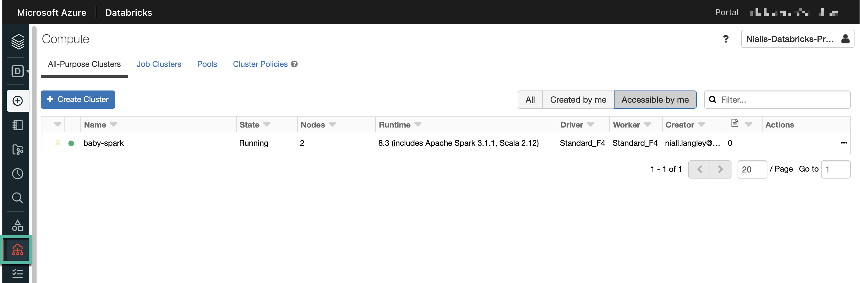
Once you have the jar file downloaded, we need to add it to our Databricks cluster. In Databricks, navigate to the Compute tab and select the cluster you want to install the library onto. Make sure it’s up and running too.
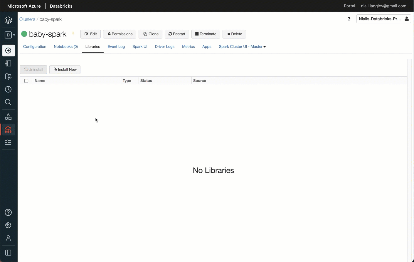
Go to the Libraries tab, and click add. Drag your downloaded jar file into the popup window and click Install.
Python Notebook Code
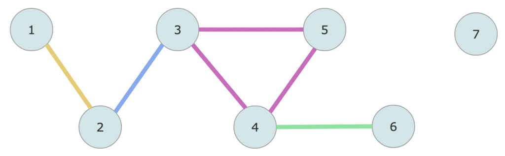
Now the library is installed, we can write some code. We’ll create a DataFrame from an array to give us the same data as in the previous posts. As a refresher, our data looks like this:
| Id | Supplier Name | Tax Number | Bank Sort Code | Bank Account Number | Required Output |
| 1 | AdventureWorks Ltd. | 12345678 | 02-11-33 | 12345678 | 1 |
| 2 | AdventureWorks | 12345678 | 02-55-44 | 15161718 | 1 |
| 3 | ADVENTURE WORKS | 23344556 | 02-55-44 | 15161718 | 1 |
| 4 | DVENTURE WORKS LTD. | 23344556 | 02-77-66 | 99887766 | 1 |
| 5 | AW Bike Co | 23344556 | 02-88-00 | 11991199 | 1 |
| 6 | Big Bike Discounts | 55556666 | 02-88-00 | 11991199 | 1 |
| 7 | Contoso Corp | 90009000 | 02-99-02 | 12341234 | 2 |
This produces the same simple disconnected graphs as last time. We have one graph with 6 nodes, and another graph with a single node.
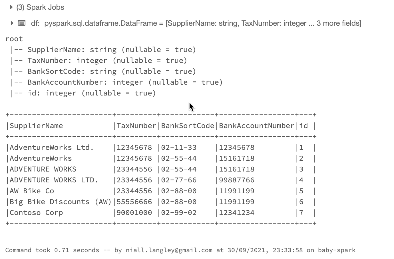
And here’s the python to create a DataFrame with the data above, and then show us the schema and the data. Add this to the first cell in your notebook.
from pyspark.sql.functions import *
from pyspark.sql.types import StructType,StructField, StringType, IntegerType
from pyspark.sql.window import Window

# Create the data as an array
data = [
  ("AdventureWorks Ltd.",      12345678, "02-11-33", 12345678),
  ("AdventureWorks",           12345678, "02-55-44", 15161718),
  ("ADVENTURE WORKS",          23344556, "02-55-44", 15161718),
  #("ADVENTURE WORKS BIKES",    23344556, "02-55-44", 15161718),
  ("ADVENTURE WORKS LTD.",     23344556, "02-77-66", 99887766),
  ("AW Bike Co",               23344556, "02-88-00", 11991199),
  ("Big Bike Discounts (AW)",  55556666, "02-88-00", 11991199),
  ("Contoso Corp",             90001000, "02-99-02", 12341234),
]

# Create the schema
schema = StructType([
    StructField("SupplierName",StringType(),True),
    StructField("TaxNumber",IntegerType(),True),
    StructField("BankSortCode",StringType(),True),
    StructField("BankAccountNumber", IntegerType(), True)
  ])

# Use the data array and schema to create a dataframe
df = spark.createDataFrame(data=data,schema=schema)

# We need a row id added to make building a graph simpler, so add that using a window and the row\_number function
windowSpec = Window().partitionBy(lit('A')).orderBy(lit('A'))
df = df.withColumn("id", row_number().over(windowSpec))

#Finally show the schema and the results
df.printSchema()
df.show(truncate=False)
So what have we done there? We created an array and a schema, and then used those to create a DataFrame. We added a new column to the DataFrame with a sequential number (using the window function row_number()) so we have a nice simple node id for building a graph. The name of the id column must be id in lowercase to work with the GraphFrame later.
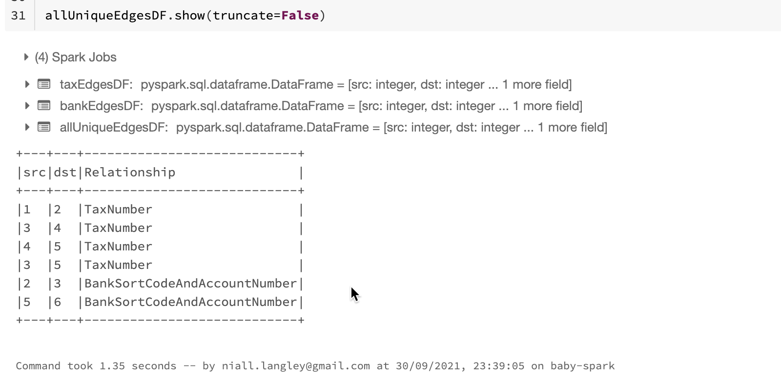
Add another cell to to the notebook and add the following code to build the edges DataFrame.
# Create a data frame for the edges, by joining the data to itself. We do this once for the TaxNumber column
# and then again for the BankSortCode and BankAccountNumber columns, and union the results

# We are building a bidirectional graph (we only care if nodes are joined), so we make sure the left RowId > right RowId
# to remove duplicates and rows joining to themselves
taxEdgesDF = (df.alias("df1")
    .join(df.alias("df2"),
        (col("df1.TaxNumber") == col("df2.TaxNumber"))
        & (col("df1.id") > col("df2.id")),
        "inner"
    )
    .select(least("df1.id", "df2.id").alias("src"),
        greatest("df1.id", "df2.id").alias("dst")
    )
    .withColumn("Relationship", lit("TaxNumber"))
)

bankEdgesDF = (df.alias("df1")
    .join(df.alias("df2"),
        (col("df1.BankSortCode") == col("df2.BankSortCode"))
        & (col("df1.BankAccountNumber") == col("df2.BankAccountNumber"))
        & (col("df1.id") > col("df2.id")),
        "inner"
    )
    .select(least("df1.id", "df2.id").alias("src"),
        greatest("df1.id", "df2.id").alias("dst")
    )
    .withColumn("Relationship", lit("BankSortCodeAndAccountNumber"))
)

allUniqueEdgesDF = taxEdgesDF.union(bankEdgesDF)

allUniqueEdgesDF.show(truncate=False)
This is just joining the nodes to the other nodes in the same way as the join in the CTE method did. We join nodes based on the tax number, or the composite bank details columns. We limit the join to nodes where the id of the first node is larger than the id of the second node, as we don’t want nodes to join to themselves, and the edges are not directional.
Now we can add another cell to create the GraphFrame, and print some simple information about node and edge counts. Note that we have to call the cache() method on the GraphFrame before we can access the nodes and edges to count them.
from graphframes import *

connectionsGF = GraphFrame(df, allUniqueEdgesDF)
connectionsGF.cache()

print("Total Number of Suppliers: " + str(connectionsGF.vertices.count()))
print("Total Number of Relationships/Types: " + str(connectionsGF.edges.count()))
print("Unique Number of Relationships: " + str(connectionsGF.edges.groupBy("src", "dst").count().count()))
Ok, so we have the GraphFrame, so how do we get the groups? Add the following code to another cell.
spark.sparkContext.setCheckpointDir("/tmp/checkpoints")

connectedComponents = connectionsGF.connectedComponents()
connectedComponents.where("component != 0").show()
We use the GraphFrame function connectedComponents() to get the groupings We have to set the spark context checkpoint directory before we use the connected components function. The component column is the group id from the graph function.
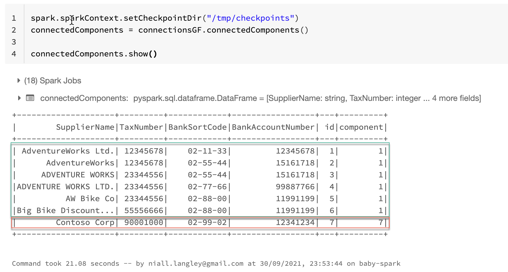
I didn’t write the results out to storage in this example, but the results are a normal spark DataFrame, so it would be easy enough to write them out to a delta table.
Conclusions
We can see from this that if we are working with our data in Spark and Synapse SQL pools, we still have option to do associative grouping. The functions did not seem the quickest with only a small amount of data, and I’ve not tested how the performance scales, especially with multiple workers. Will we get lots of shuffling of data, I’m not sure but that sounds like something interesting to explore. It’s probably a good idea to do this kind of grouping once up front if you can though, rather than calculating it on demand, as the processing for it is likely to be quite intensive.
I did try and get the ode running in a Synapse Spark Pool notebook, but I could not get python to see the library once I had added the jar file to the workspace. It seems like Synapse is happy to use python wheels, but not jar files (Scala / Java) libs. Converting the code to Scala did work though, so maybe I’m missing something there. If you do manage to get that working, let me know in the comments.